A survey of database storage engines

What and why

There’s plenty of material online about storage engines (eg see this and its follow-up).

Tl;dr:

• A storage engine is the component of a database that handles CRUD operations, interfacing with the underlying memory and storage systems. It usually relies on two primary types of indexes: B+trees and Log-Structured Merge-Trees (LSM-trees).
• B+tree provides balanced read and write performance, while LSM-tree is optimized for high write throughput. In addition to the workload type, other factors, such as concurrency control, also have a significant impact on storage engine performance (eg see this)

My goal here is to give you a context for that summary, build on top of it and shallowly sketch the current storage-engine landscape.

Background

From the 1970s through the 1980s, a major use case for databases was recording interactive business transactions (eg airline bookings). These use cases, now classified as OLTP, consist of many short reads and/or writes that touch only a few records (or rows) at a time. On the hardware of the time, performance was dominated by the mechanical latency of hard disks (explained next). To cope with this, databases were built to minimize random I/O, using B+tree indexes as the standard on-disk data structure and a buffer manager to cache frequently accessed disk pages in memory.

As data volumes grew through the 1990s and 2000s, users wanted systems that could answer analytical questions (eg what are the top 3 best-selling products in North America in Q2?). These workloads, now called OLAP, stressed the system in a different way: instead of random-seek latency, the main bottleneck was wasted I/O bandwidth caused by reading entire rows when only a few columns (eg productId, sold count, location, time) were needed. This drove the adoption of columnar storage layouts, which allow engines to read only the referenced columns and exploit high sequential throughput.

Stepping back, every storage engine navigates a fundamental trade-off between three costs:

• Write amplification: bytes written to storage per byte of user data. A value of 10× means 10 bytes hit disk for every 1 byte from the application.
• Read amplification: bytes read from storage per byte of requested data.
• Space amplification: bytes stored in storage per byte of user data.

No design optimizes all three. B+trees are read-optimized at the cost of higher write amplification. LSM-trees are write-optimized at the cost of higher read and space amplification. Understanding this trifecta requires understanding the underlying storage hardware (next section), then examining how OLTP and OLAP engines navigate these trade-offs.

Storage Hardware

The above trade-offs are heavily influenced by the the underlying storage hardware and its so-called memory hierarchy.

The figure belowSee “Persistent Memory Primer” (Oracle Database Insider, 2020). illustrates the different types of storage hardware currently in use, highlighting the trade-offs between performance, capacity, and price. One of the key principles of the memory hierarchy is that lower latency hardware is inevitably more expensive and limited in capacity.

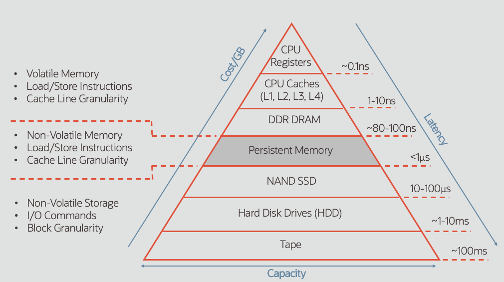
Registers sit at the very top of the hierarchy, providing the CPU with the fastest possible access to data.

CPU caches follow immediately after. Most modern CPUs employ a multi-level cache hierarchy (L1, L2, and often L3).

• L1: Located closest to the CPU core, L1 offers the highest speed. It is usually split into instruction-specific (I-cache) and data-specific (D-cache) units.
• L2 & L3: L2 is physically separate and slightly slower, while L3 is generally shared across multiple cores.

Cache memory is typically implemented using SRAM (Static Random Access Memory). SRAM requires multiple transistors to store a single bit, making it faster to read and write but also more expensive and less dense than DRAM (Dynamic Random Access Memory).

Main Memory (RAM) is the primary storage directly accessible to the CPU via the memory bus. The CPU fetches instructions and active data from here. Main memory is usually implemented with DRAM, which uses only one transistor and one capacitor per bit, allowing for higher density at a lower cost than SRAM.

Non-volatile Storage has a rich history, largely dominated by Hard Disk Drives (HDDs) until recentlySee “Mass Storage” (Wikipedia).. HDDs read and write data using a magnetic read-write head that floats just nanometers above a rapidly spinning, magnetically-coated platter, as shown below.

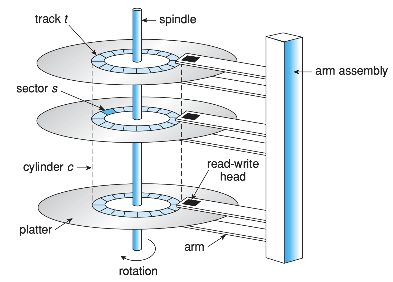
The mechanical nature of HDDs imposes physical latency limits. This is why Solid State Drives (SSDs)—based on 3D NAND flash with no moving parts—have largely overtaken HDDs for many use cases. SSDs offer a massive performance leap, providing over 1,000x better random read/write IOPS than HDDs with similar or better power efficiency. However, they introduce their own specific complexitiesSee Alibaba Cloud Storage Team, “Storage System Design Analysis: Factors Affecting NVMe SSD Performance (1)” (Alibaba Cloud Community, 2019).:

• Read/Write Asymmetry: While reads are fast, writes can degrade over time. SSDs cannot overwrite a single page (eg 4KB) directly; they must erase an entire block (eg 128 pages) to reuse it. This requires relocating valid data to a new block before erasing the old one—a process known as “Write Amplification.”

• Service Life: NAND flash cells withstand a finite number of program/erase cycles before failing. The internal Garbage Collection (GC) process required to manage blocks further contributes to this wear.

Performance metrics for random and sequential accessSSD performance is typically measured at Queue Depth 32 (QD-32).:

• HDD:
  • Random Reads (4KB): ~100 IOPS (~10ms latency).
  • Sequential Reads: ~40k IOPS (~150 MB/s throughput).
• SSD (QD-32):
  • Random Reads (4KB): ~100k IOPS (SATA) to ~1M IOPS (NVMe PCIe 5).
  • Random Writes (4KB): ~80k IOPS (SATA) to ~800k IOPS (NVMe PCIe 5).
  • Sequential Reads: ~125k IOPS (SATA) to ~3.5M IOPS (NVMe PCIe 5). In throughput terms, ~500 MB/s (SATA) to ~14 GB/s (NVMe PCIe 5). Note that throughput is often bottlenecked by the interconnect (bus).

Emerging persistent memory technologies bridge the gap between volatile RAM and non-volatile storage. They combine the durability of storage with the byte-addressable access speeds of traditional RAMSee Dimitrios Koutsoukos et al., “How to Use Persistent Memory in Your Database” (arXiv, 2021)..

These hardware characteristics directly shaped storage engine design:

• B+trees minimize random I/O, critical when HDDs dominated.
• LSM-trees convert random writes to sequential, exploiting SSD strengths.
• Columnar layouts reduce I/O by reading only the columns a query references..

OLTP

Shopping on an e-commerce site is a balanced read-write OLTP workload, involving browsing specific products (reads) and placing orders (writes). Application logging is write-heavy, requiring higher write throughput. IoT sensor ingestion is write-extreme, demanding the highest write throughput.

While all of these are OLTP use cases, their vastly different write requirements are best served by different storage engine designs. For example:

• B+tree-based: ideal for balanced read-write workloads.
• LSM (Log-Structured Merge) tree-based: optimized for write-heavy workloads.
• LSH (Log-Structured Hash) table-based: designed for extremely high-ingest workloads.

B+tree-based

Introduced in the early 1970sSee Rudolf Bayer and Edward McCreight, “Organization and Maintenance of Large Ordered Indices” (ACM SIGFIDET, 1970).See Ben Dicken, “B-Trees and Database Indexes” (PlanetScale, 2024).See Ben Congdon, “B-Trees: More Than I Thought I’d Want to Know” (2021)., the B+tree maintains global sorted order via a self-balancing tree and in-place updates. It serves as the foundational data structure for primary and secondary indexes in most relational databases.

MySQL’s InnoDB is a good example of a B+tree-based storage engine. Its architectureSee “InnoDB Architecture” (MySQL 9.5 Reference Manual). is shown below. File-Per-Table Tablespaces is where table data and indexes are stored.

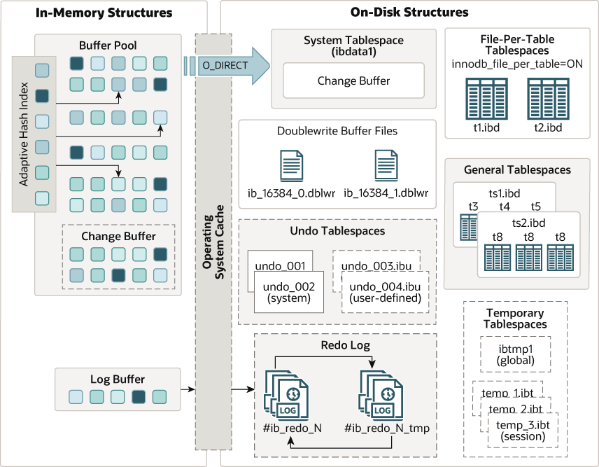
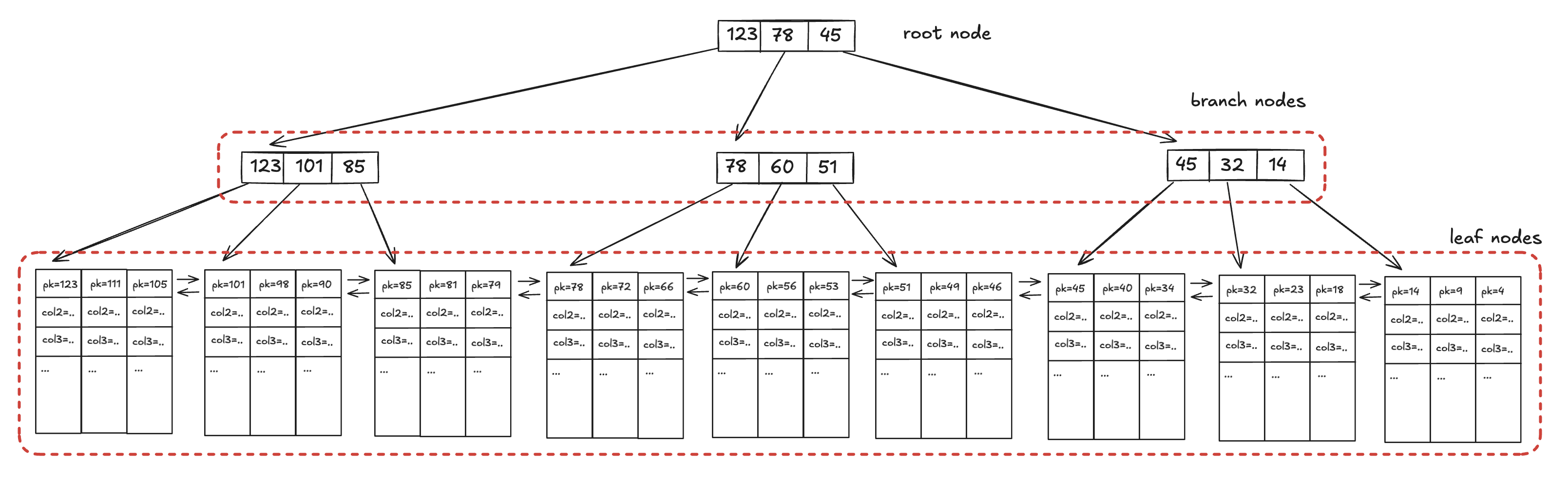
With file-per-table enabled, each .ibd file stores the table’s clustered index and all its secondary indexesSee Jeremy Cole, “The Basics of InnoDB Space File Layout” (2013).. InnoDB clusters the table on the primary key: the leaf pages of the primary B+tree contain entire rows, ordered by that key. Secondary indexes store indexed key values plus primary-key columns as the row locator. The figure below shows a simplified primary index layout.

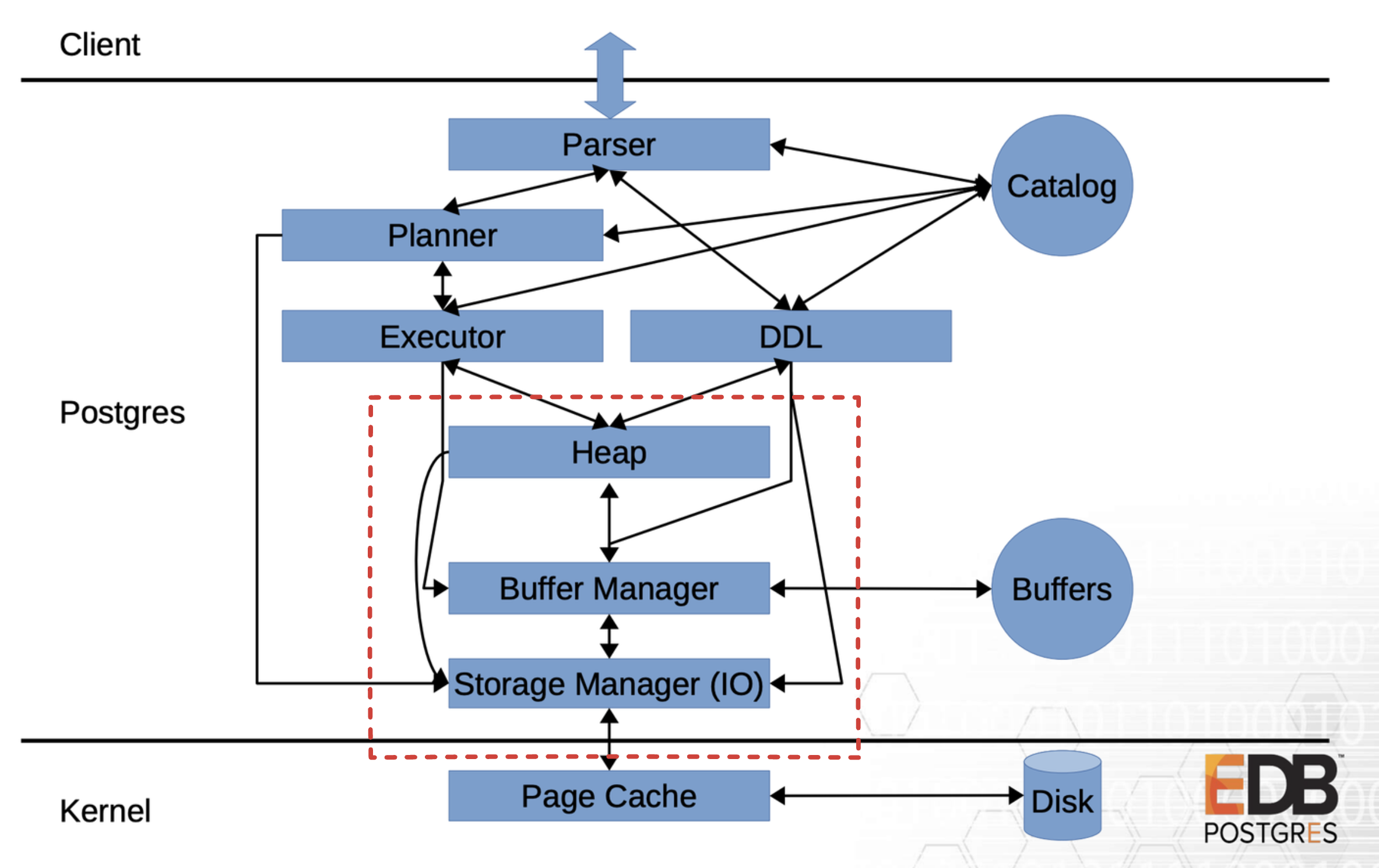
PostgreSQL uses the same B+tree structure for indexes but stores table data separately in heap files (unordered pages where rows can be inserted anywhere there is free space). Indexes live in their own files. PostgreSQL’s architectureSee Andres Freund, “Pluggable Table Storage in PostgreSQL” (PGVision, 2019). is shown below; the dashed red box marks its storage engine.

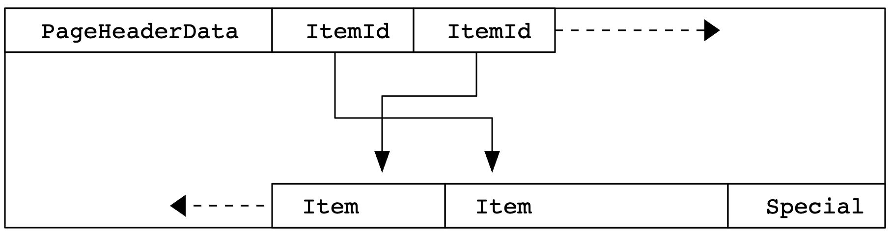
Each Postgres table or index is stored in its own file, accompanied by two additional forks for the free space map (FSM) and visibility map (VM). Tables larger than 1GB are split into 1GB segments (name.1, name.2, etc.) to accommodate filesystem limits. The main fork is divided into 8KB pages; for heap tables, all pages are interchangeable, so a row can be stored anywhere. Indexes dedicate the first block to metadata and maintain different page types depending on the access method. The generic page layout is shown below:

By default, a primary key or unique constraint creates a B+tree index, so you typically end up with at least one file per table plus at least one more for its B+tree index. The figure below shows how the table and its B+tree primary index are related.

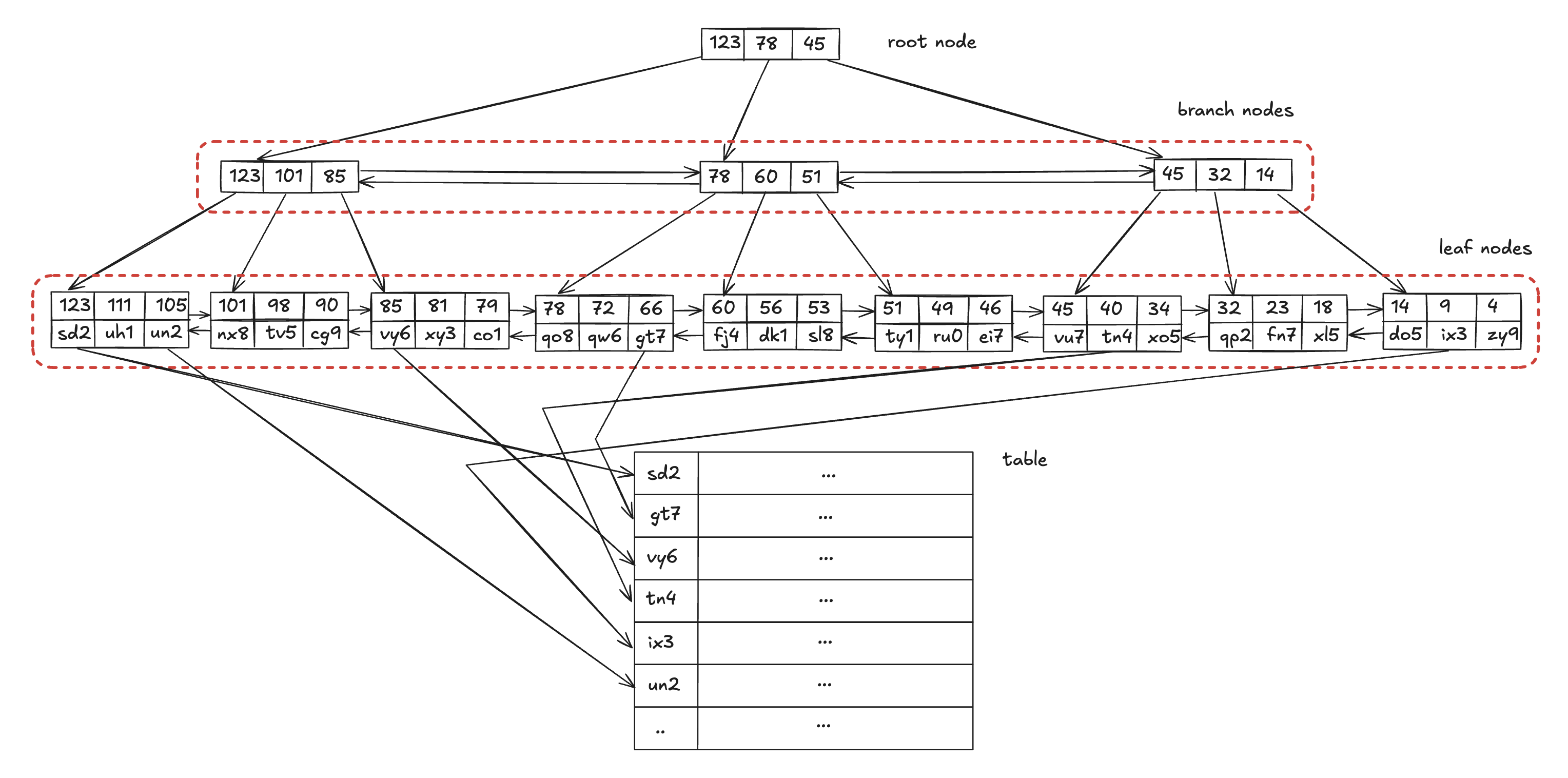
Unlike InnoDB’s clustered index, where leaf pages contain entire rows, PostgreSQL’s B+tree leaf pages store (key, TID) pairs. The TID (tuple identifier) is a pointer to the row’s physical location in the heap. Secondary indexes work the same way where they store TIDs pointing directly to heap tuples, rather than going through the primary key as in MySQL. This means every index lookup, whether primary or secondary, requires a separate heap fetch to retrieve the actual row data. This design simplifies index management but contributes to the MVCC-related bloat discussed in the CMU article linked earlier.

LSM-tree-based

The Log-Structured Merge (LSM) tree was introduced in academic literature in 1996. LSM storage engines buffer writes in memory, periodically flush sorted runs to disk, and merge those runs in the background. This trades the strict in-place updates and globally ordered layout of B+trees for batched sequential I/O, yielding much higher write throughput. The trade-off is extra read latency (eg short-range lookups may hit multiple levels) and higher space/memory amplificationSee Stratos Idreos and Mark Callaghan, “Key-Value Storage Engines” (ACM SIGMOD, 2020)..

RocksDB is one of the state-of-the-art LSM-tree based storage engines. See its wiki for details.

LSH-table-based

The Log-Structured Hash (LSH) tables push the LSM idea to its extreme by dropping order maintenance entirely. Instead, they rely on an in-memory index, eg hash table, for efficient key-value lookups. New records are buffered in memory and then flushed to disk as new segments in a single, ever-growing log.

This design makes writes almost entirely sequential, supporting extremely high ingest rates. The main downsides are inefficient range scans, which must either scan multiple log segments or resort to a full table scan, and higher memory amplification compared to LSM-trees, as the in-memory index must hold all keysSee Stratos Idreos and Mark Callaghan, “Key-Value Storage Engines” (ACM SIGMOD, 2020).. Faster and its follow ups are good examples of such a systemSee Badrish Chandramouli et al., “FASTER: A Concurrent Key-Value Store with In-Place Updates” (ACM SIGMOD, 2018)..

Buffering Semantics Across OLTP Storage Engines

A buffer manager’s importance differs sharply across these storage-engine families.

In B+tree-based engines, the buffer pool is critical. All reads and all in-place writes go through it, making it the main sync point. Eviction and dirty-page scheduling materially affect performance because B+trees repeatedly touch a small, high-reuse working set (root, internal nodes, hot leaves).

In LSM-tree-based engines, buffering isn’t in the write path. Read performance still depends heavily on caching (block cache, filter/index block cache).

In LSH-table-based designs, the buffer manager’s role shrinks further. These systems use append-only segments and in-memory hash indexes and typically lean on the OS page cache rather than a database buffer pool. Caching still mitigates read amplification, but the engine’s own buffering layer is minimal.

OLAP

The logical access pattern of an OLAP system typically involves scanning specific columns across millions of rows, rather than retrieving all columns for a few specific rows. Consequently, these systems use a column-oriented format, storing values from each column contiguously.

In practice, however, storage engines rarely use a pure columnar approach. Because queries often filter by a specific range (eg time), engines use a hybrid layout. The table is horizontally partitioned into blocks of rows (often called row groups), and within those blocks, column values are stored separately. This is illustrated in the image belowSee Vu Trinh, “We Might Not Fully Understand the Column Store!” (2024)..

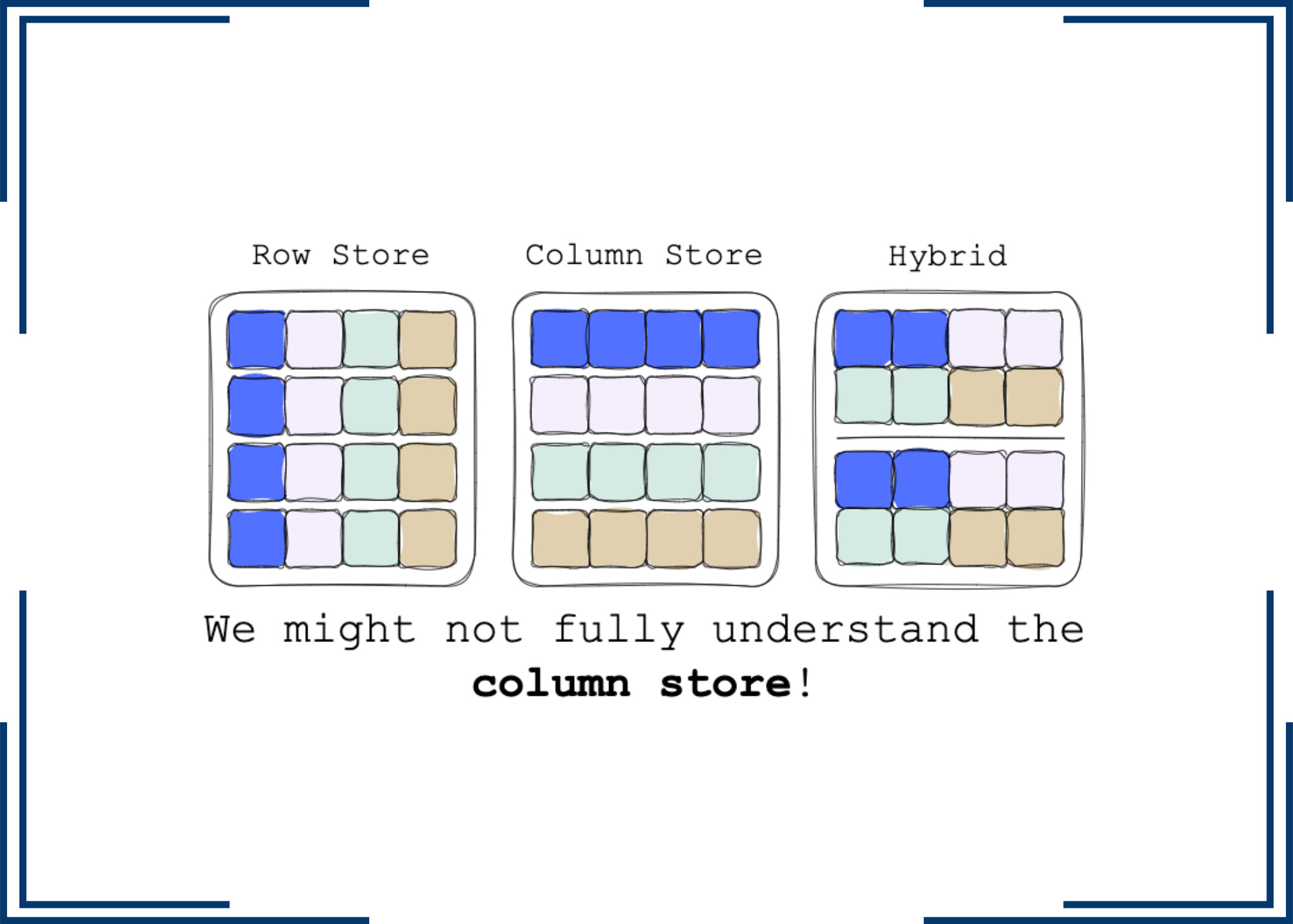
This hybrid layout allows the engine to be surgical, fetching only the specific row groups required for a query. Within each row group, all columns store values in the same positional row order, so the engine can reconstruct rows by aligning the i-th value across columns. Because OLAP systems must frequently reassemble rows, this positional structure is essential.

Most OLAP engines use this hybrid layout idea as a foundation, customizing it for their query engines while supporting Parquet and ORC for cross-platform data sharingSee Xinyu Zeng et al., “An Empirical Evaluation of Columnar Storage Formats” (PVLDB, 2023)..

One of the major advantages of this layout is compression. Since data within a column is uniform (eg a column of integers), it compresses significantly better than row-oriented data. See this for a list of potential compressions.

The Metadata Hierarchy

In modern OLAP architectures, raw data files are wrapped in additional layers of metadata (eg to support ACID transactionsSee Xinyu Zeng et al., “An Empirical Evaluation of Columnar Storage Formats” (PVLDB, 2023).):

• Table Formats: These files track which data files belong to a specific table, manage schemas, and store file-level statistics (min/max values). Apache Iceberg and Databricks’ Delta are the industry standards here.
• Data Catalogs: This layer sits above table formats, defining which tables constitute a database and handling namespace operations like creating, renaming, or dropping tables. Snowflake’s Polaris and Databricks’ Unity Catalog are common examples.

Handling Writes

While columnar storage is excellent for reading, it is inefficient for writing individual rows, particularly in sorted tables. To address this, OLAP systems typically use a log-structured approach.

Writes are first directed to a row-oriented, sorted, in-memory buffer (often called a memtable). When this buffer fills, the data is sorted, converted to the columnar format, and flushed to disk as a new immutable file. Because files are written in bulk and never modified in place, object storage is an ideal backend for this architecture.

During a read, the query engine examines both the columnar data on disk and the recent writes in the memory buffer, merging the two results seamlessly so the user sees a consistent view of the data.

Modern Storage APIs

Modern storage APIs are an important area today because their cost is one of the performance bottlenecks. For example, when storage took say 10,000 µs (HDD), a 5 µs software delay was invisible (0.05%). Now that storage takes 10 µs (SSD), that same fixed 5 µs software delay is a massive bottleneck (33%).

The diagram below shows the currently available Linux storage I/O interfacesSee Gabriel Haas and Viktor Leis, “What Modern NVMe Storage Can Do, and How to Exploit It: High-Performance I/O for High-Performance Storage Engines” (PVLDB, 2023)..

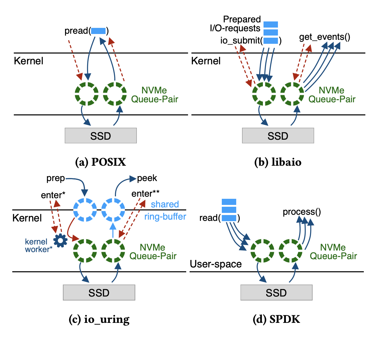
POSIX defines synchronous and asynchronous I/O. With synchronous I/O, a pread() call blocks your thread until the data is ready. With asynchronous I/O, an aio_read() returns immediately while a user-space helper thread (spawned by glibc) performs the blocking call in the background. With buffered I/O, both modes pay the same costs: one system call per request and two data copies (device → kernel → user). If you open the file with O_DIRECT, the kernel bypasses the page cache and copies data directly from the device into user space, avoiding the second copy. Most databases use synchronous I/O with O_DIRECT for this reason (more?).

In libaio, asynchrony is handled in the kernel. You call io_submit() to queue one or more requests; the call returns immediately while the kernel executes the I/O. You later call io_getevents() to collect completions. libaio is almost always used with O_DIRECT to avoid the extra copy through the page cache. In this case, the effective cost is two system calls per I/O request: one to submit and one to get completions.

io_uring is a new Linux I/O interface designed to be easy and efficient to use. It introduces a submission and completion queue pair that an application can use to communicate with the kernel for doing I/O. This means no metadata-copy overhead that POSIX and libaio pay by default. Its main modes of operation are shown belowSee Diego Didona et al., “Understanding Modern Storage APIs: A Systematic Study of libaio, SPDK, and io-uring” (ACM SYSTOR, 2022)..

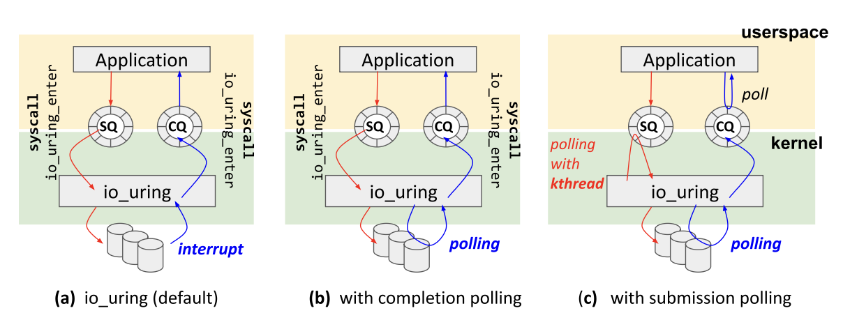
• (a) The application writes a request into the submission queue (SQ) and issues io_uring_enter() to notify the kernel. The kernel performs the I/O asynchronously and posts results into the completion queue (CQ). The application calls io_uring_enter() again to wait for completions. This still costs two syscalls per request but avoids the metadata copy.
• (b) Same as (a), but the application tells the kernel to poll the hardware instead of relying on interrupts when communicating with the SSD driver.
• (c) io_uring can eliminate both syscalls by creating a dedicated kernel thread per io_uring context. That thread polls the SQ, and the application polls the CQ. The tradeoff is the extra kernel thread.

io_uring supports buffered (involves OS page cache), unbuffered (O_DIRECT) and passthrough I/O (bypassing the generic storage stack).

SPDK bypasses the kernel entirely by mapping NVMe queues into user space, allowing applications to issue commands directly to the device. While this approach maximizes performance, it complicates integration with storage engines that rely on other kernel services. Furthermore, SPDK requires exclusive control of the physical device, rendering it unfeasible for most production environments.

Conclusion

This was mostly a summary post to clarify my own understanding of the current storage engine landscape.

A few observations:

• Hardware: NVMe SSDs have shifted the bottleneck from mechanical latency to software overhead.
• Storage APIs: io_uring is emerging as the standard for high-performance async I/O, eliminating the syscall overhead that POSIX and libaio impose.
• Data structures: Increasingly write-heavy workloads (application logging, IoT ingestion) have pushed the field from B+trees toward LSM-trees and LSH-tables. That said, existing engines also invest in optimizing for the opposite direction—LSM-trees add Bloom filters, fence pointers and compaction optimizations for better reads; B+tree variants adopt log-structured techniques for better writes.
• OLAP: The field has standardized on layered abstractions—columnar formats (Parquet, ORC), table formats (Iceberg, Delta), and catalogs—each solving a distinct problem. Write handling borrows log-structured techniques from OLTP.

Public cloud infrastructureSee Till Steinert, Maximilian Kuschewski, and Viktor Leis, “Cloudspecs: Cloud Hardware Evolution Through the Looking Glass” (CIDR, 2026). may be another force reshaping this landscape, though that’s beyond the scope of this post.